Why Are the Features Obtained by "Predict" and "Forward" Function Very Different?

Posted by TheMatrix on 2020-07-11

       本博客主要内容本应该是我提出的issue被广泛讨论的,所以写成英文方便国外网友讨论,后来干脆整理成了一篇博客,依旧保留了英文模式,逐步引人入思,遂成文,发之,英文表达有不妥之处,敬请谅解!

According to official instructions, “forward” is used for inference during the network training phase, and “predict” is used for inference during the network prediction phase.But there are a large number of networks used by the batchnorm layer,the features of forward and predict are very different.

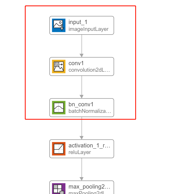
       For convenience, only observe the output features of the first convolution layer and bathhorm layer of resnet50,We first take the resnet50 network provided by matlab as an example to illustrate, convert to dlnetwork and compare.

1
2
3
4
5
6
7
net50 = resnet50;
inputsize = [224,224];
img = imresize(imread('peppers.png'),inputsize);
inputImg = dlarray(im2single(img),'SSCB');
lg = layerGraph(net50);
newlg = removeLayers(lg,'ClassificationLayer_fc1000');
dlnet = dlnetwork(newlg); % take long time ???

fig

network

simple case

       We extract the feature named “fc1000_softmax” layer,big different features between forward_f and predict_f ?

1
2
[forward_f,state1] = forward(dlnet,inputImg);
[~,ind1] = max(forward_f)
1
2
3
ind1 = 
1(C) x 1(B) dlarray
464
1
2
[predict_f,state2] = predict(dlnet,inputImg);
[~,ind2] = max(predict_f)
1
2
3
ind2 = 
1(C) x 1(B) dlarray
917
1
2
activations_f = activations(net50,im2single(img),'fc1000_softmax','OutputAs','columns');
[~,ind3] = max(activations_f)
1
ind3 = 917
1
2
3
dlnet.State = state1;
[predict_update_f,state4] = predict(dlnet,inputImg);
[~,ind4] = max(predict_update_f)
1
2
3
ind4 = 
1(C) x 1(B) dlarray
665

Why is forward_f and predict_f very different? Then we look at the following step by step analysis why this is so!

analysis

Calculate whether the output of the BN layer is consistent in two ways

       forward_features{1} are convolution features, forward_features{2} are features from batchnorm.

1
2
3
4
5
6
7
8
9
10
11
12
Epsilon = 1e-4;
convlayer = dlnet.Layers({dlnet.Layers.Name}=="conv1");
bnlayer = dlnet.Layers({dlnet.Layers.Name}=="bn_conv1");

forward_features = cell(2,1);
[forward_features{:},state]= forward(dlnet,inputImg,'Outputs',{'conv1','bn_conv1'});
[dlY,mu,sigmasq] = batchnorm(forward_features{1},squeeze(bnlayer.Offset),...
squeeze(bnlayer.Scale),100*ones(64,1),2*ones(64,1));% ,squeeze(bnlayer.TrainedMean),squeeze(bnlayer.TrainedVariance) ,squeeze(dlnet.State.Value{1}),squeeze(dlnet.State.Value{2})
if ~all(abs(forward_features{2}-dlY)<Epsilon,'all')
forward_features{2}(1:10,1:10,1)
dlY(1:10,1:10,1)
end
1
2
3
4
5
6
7
8
9
10
11
12
13
14
15
16
17
18
19
20
21
22
23
24
ans = 
10x10 single dlarray
-7.5244 6.2767 4.6619 4.6621 4.6618 4.6639 4.6621 4.6621 4.6631 4.6623
-11.4266 0.7695 -0.0690 -0.0695 -0.0698 -0.0709 -0.0674 -0.0705 -0.0695 -0.0680
-8.8744 2.5809 1.5790 1.5792 1.5807 1.5787 1.5793 1.5794 1.5794 1.5802
-8.8747 2.5823 1.5794 1.5783 1.5799 1.5800 1.5780 1.5790 1.5786 1.5789
-8.8757 2.5821 1.5797 1.5781 1.5799 1.5802 1.5795 1.5788 1.5793 1.5789
-8.8753 2.5799 1.5809 1.5800 1.5775 1.5789 1.5800 1.5802 1.5793 1.5794
-8.8744 2.5816 1.5757 1.5819 1.5810 1.5768 1.5765 1.5796 1.5796 1.5780
-8.8748 2.5841 1.5780 1.5761 1.5814 1.5807 1.5780 1.5772 1.5791 1.5797
-8.8753 2.5818 1.5814 1.5788 1.5785 1.5790 1.5807 1.5798 1.5780 1.5786
-8.8745 2.5813 1.5785 1.5802 1.5790 1.5781 1.5792 1.5799 1.5793 1.5791
ans =
10x10 single dlarray
-7.5244 6.2767 4.6619 4.6621 4.6618 4.6639 4.6621 4.6621 4.6631 4.6623
-11.4266 0.7695 -0.0690 -0.0695 -0.0698 -0.0709 -0.0674 -0.0705 -0.0695 -0.0680
-8.8744 2.5809 1.5790 1.5792 1.5807 1.5787 1.5793 1.5794 1.5794 1.5802
-8.8748 2.5823 1.5794 1.5783 1.5799 1.5800 1.5780 1.5790 1.5786 1.5789
-8.8757 2.5821 1.5797 1.5781 1.5799 1.5802 1.5795 1.5788 1.5793 1.5789
-8.8753 2.5799 1.5809 1.5800 1.5775 1.5789 1.5800 1.5802 1.5793 1.5794
-8.8744 2.5816 1.5757 1.5819 1.5810 1.5768 1.5765 1.5796 1.5796 1.5780
-8.8749 2.5841 1.5780 1.5761 1.5814 1.5807 1.5780 1.5772 1.5791 1.5797
-8.8753 2.5818 1.5814 1.5788 1.5785 1.5790 1.5807 1.5798 1.5780 1.5786
-8.8745 2.5813 1.5785 1.5802 1.5790 1.5781 1.5792 1.5799 1.5793 1.5791

There is data output, indicating different, but the data looks the same, why?

Than test the mean of “forward” function and batchnorm() function update

1
2
3
4
5
temp = squeeze(state.Value{1});
if ~all(mu==temp,"all")
mu(1:10)
temp(1:10)
end
1
2
3
4
5
6
7
8
9
10
11
12
13
14
15
16
17
18
19
20
21
22
23
ans = 10x1 single column vector    
86.4990
88.6642
83.5626
90.9294
90.6073
97.3961
81.3441
96.4360
71.8466
90.3925

ans = 10x1 single column vector
-6.7745
-3.0580
-12.7130
2.2173
1.1940
12.9555
-16.8975
12.7977
-33.9066
0.6955

No result output, indicating that the mean of “forward” function is equal to batchnorm() function update.
Than test the variance of “forward” function and batchnorm() function update

1
2
3
4
5
temp = squeeze(state.Value{2});
if ~all(abs(sigmasq - temp)<Epsilon,"all")
sigmasq(1:10)
temp(1:10)
end
1
2
3
4
5
6
7
8
9
10
11
12
13
14
15
16
17
18
19
20
21
22
23
24
25
ans = 10x1 single column vector    
50.6704
1.9740
4.0529
12.4677
8.9267
4.2635
8.7056
37.6846
3.5269
2.0079

ans = 10x1 single column vector
1.0e+03 *

4.5144
1.8444
1.2742
0.6138
2.7673
9.6139
2.1018
2.1818
9.7148
0.5078

There is data output, indicating different, but the data looks the same, why?

Than compare the difference between forward and predict

1
2
3
4
5
6
predict_features = cell(2,1);
[predict_features{:}]= predict(dlnet,inputImg,'Outputs',{'conv1','bn_conv1'});
if ~all(abs(forward_features{1}-predict_features{1})<Epsilon,"all") % compare conv features
forward_features{1}(1:10,1:10,1)
predict_features{1}(1:10,1:10,1)
end

No result output, indicating that the convolution operation is consistent in forward and predict results.

1
2
3
4
if ~all(abs(forward_features{2}-predict_features{2})<Epsilon,"all") % compare batchnorm features
forward_features{2}(1:10,1:10,1)
predict_features{2}(1:10,1:10,1)
end
1
2
3
4
5
6
7
8
9
10
11
12
13
14
15
16
17
18
19
20
21
22
23
24
ans = 
10x10 single dlarray
-7.5244 6.2767 4.6619 4.6621 4.6618 4.6639 4.6621 4.6621 4.6631 4.6623
-11.4266 0.7695 -0.0690 -0.0695 -0.0698 -0.0709 -0.0674 -0.0705 -0.0695 -0.0680
-8.8744 2.5809 1.5790 1.5792 1.5807 1.5787 1.5793 1.5794 1.5794 1.5802
-8.8747 2.5823 1.5794 1.5783 1.5799 1.5800 1.5780 1.5790 1.5786 1.5789
-8.8757 2.5821 1.5797 1.5781 1.5799 1.5802 1.5795 1.5788 1.5793 1.5789
-8.8753 2.5799 1.5809 1.5800 1.5775 1.5789 1.5800 1.5802 1.5793 1.5794
-8.8744 2.5816 1.5757 1.5819 1.5810 1.5768 1.5765 1.5796 1.5796 1.5780
-8.8748 2.5841 1.5780 1.5761 1.5814 1.5807 1.5780 1.5772 1.5791 1.5797
-8.8753 2.5818 1.5814 1.5788 1.5785 1.5790 1.5807 1.5798 1.5780 1.5786
-8.8745 2.5813 1.5785 1.5802 1.5790 1.5781 1.5792 1.5799 1.5793 1.5791
ans =
10x10 single dlarray
-1.8324 2.4990 1.9922 1.9922 1.9921 1.9928 1.9923 1.9922 1.9926 1.9923
-3.0570 0.7706 0.5074 0.5073 0.5072 0.5068 0.5080 0.5070 0.5073 0.5078
-2.2560 1.3391 1.0246 1.0247 1.0252 1.0245 1.0247 1.0248 1.0248 1.0250
-2.2562 1.3395 1.0248 1.0244 1.0249 1.0250 1.0243 1.0247 1.0245 1.0246
-2.2564 1.3395 1.0249 1.0244 1.0249 1.0250 1.0248 1.0246 1.0247 1.0246
-2.2563 1.3388 1.0252 1.0250 1.0242 1.0246 1.0250 1.0250 1.0248 1.0248
-2.2561 1.3393 1.0236 1.0256 1.0253 1.0240 1.0239 1.0248 1.0249 1.0243
-2.2562 1.3401 1.0244 1.0237 1.0254 1.0252 1.0243 1.0241 1.0247 1.0249
-2.2563 1.3394 1.0254 1.0246 1.0245 1.0247 1.0252 1.0249 1.0243 1.0245
-2.2561 1.3392 1.0245 1.0250 1.0247 1.0244 1.0247 1.0249 1.0247 1.0247

The problem is coming, the values of predict and forward are obviously different. So I want to test why predict is very different. Below I use batchnorm() function to execute the result of the last convolution, without entering mean and variance.

1
2
predict_y = batchnorm(forward_features{1},squeeze(bnlayer.Offset),squeeze(bnlayer.Scale));
predict_y(1:10,1:10,1)
1
2
3
4
5
6
7
8
9
10
11
12
ans = 
10x10 single dlarray
-7.5244 6.2767 4.6619 4.6621 4.6618 4.6639 4.6621 4.6621 4.6631 4.6623
-11.4266 0.7695 -0.0690 -0.0695 -0.0698 -0.0709 -0.0674 -0.0705 -0.0695 -0.0680
-8.8744 2.5809 1.5790 1.5792 1.5807 1.5787 1.5793 1.5794 1.5794 1.5802
-8.8748 2.5823 1.5794 1.5783 1.5799 1.5800 1.5780 1.5790 1.5786 1.5789
-8.8757 2.5821 1.5797 1.5781 1.5799 1.5802 1.5795 1.5788 1.5793 1.5789
-8.8753 2.5799 1.5809 1.5800 1.5775 1.5789 1.5800 1.5802 1.5793 1.5794
-8.8744 2.5816 1.5757 1.5819 1.5810 1.5768 1.5765 1.5796 1.5796 1.5780
-8.8749 2.5841 1.5780 1.5761 1.5814 1.5807 1.5780 1.5772 1.5791 1.5797
-8.8753 2.5818 1.5814 1.5788 1.5785 1.5790 1.5807 1.5798 1.5780 1.5786
-8.8745 2.5813 1.5785 1.5802 1.5790 1.5781 1.5792 1.5799 1.5793 1.5791

From the output results, it is consistent with forward, why is it not the result of predict? Excuse me, what happened?(it is actually “forward()” mode)

Further testing

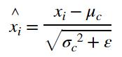
       batchnorm() is internally calculated as ,the normalized activation is calculated using the following formula:
公式1

where x_i is the input activation, μ_c(mu) and σ²(sigmaSq) are the per-channel mean and variance, respectively, and ε is a small constant. 
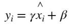
The normalized activation is offset and scaled according to the following formula:

公式2

The offset β and scale factor γ are specified with the offset and scaleFactor arguments.

1
2
3
4
5
6
7
8
9
10
11
12
13
14
15
xi = forward_features{1};% 112×112×64×1
mu_global = dlnet.State.Value{1}; % 1*1*64 "predict()" use
var_global = dlnet.State.Value{2}; % 1*1*64 "predict()" use
mu_local = mean(forward_features{1},[1,2]);% 1*1*64*1 per-channel mean, "forward()" use
var_local = var(forward_features{1},0,[1,2]);% 1*1*64*1 per-channel variance,"forward()" use

predict_mode = 0; % if the network is prediction phase
if predict_mode
norm_xi = (xi-mu_global)./sqrt(var_global+Epsilon);% 112×112×64×1, "predict()" use
else
norm_xi = (xi-mu_local)./sqrt(var_local+Epsilon);% 112×112×64×1,"forward()" use
end

cal_predict_y = bnlayer.Scale.*norm_xi+bnlayer.Offset; %112×112×64×1,Support broadcast mechanism
cal_predict_y(1:10,1:10,1)
1
2
3
4
5
6
7
8
9
10
11
12
ans = 
10x10 single dlarray
-7.5241 6.2765 4.6618 4.6619 4.6616 4.6637 4.6620 4.6620 4.6630 4.6622
-11.4261 0.7695 -0.0690 -0.0694 -0.0698 -0.0709 -0.0673 -0.0705 -0.0695 -0.0679
-8.8740 2.5809 1.5790 1.5792 1.5807 1.5787 1.5793 1.5794 1.5794 1.5802
-8.8743 2.5823 1.5794 1.5783 1.5799 1.5800 1.5780 1.5790 1.5786 1.5789
-8.8753 2.5821 1.5797 1.5781 1.5799 1.5802 1.5795 1.5788 1.5793 1.5789
-8.8749 2.5798 1.5809 1.5800 1.5775 1.5789 1.5800 1.5802 1.5793 1.5794
-8.8740 2.5815 1.5757 1.5819 1.5810 1.5768 1.5765 1.5796 1.5796 1.5780
-8.8744 2.5840 1.5780 1.5761 1.5814 1.5806 1.5779 1.5772 1.5791 1.5796
-8.8749 2.5817 1.5814 1.5787 1.5785 1.5790 1.5807 1.5798 1.5780 1.5786
-8.8741 2.5813 1.5785 1.5802 1.5790 1.5781 1.5792 1.5799 1.5793 1.5791

The results are excellent, verifying the correctness of the above results. When predict_mode=1, cal_predict_y is the same as predict_features(2); when predict_mode=0, cal_predict_y is the same as forward_features(2).

Calculate state quantity by formula

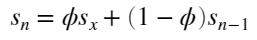
       Let’s look at a formula that is calculated and updated manually according to the formula:
公式1

where Sn is the statistic computed over several mini-batches, Sx is the per-channel statistic of the current mini-batch, and Ø is the decay value for the statistic.
       Use this syntax to iteratively update the mean and variance statistics over several mini-batches of data during training. Use the final value of the mean and variance computed over all training mini-batches to normalize data for prediction and classification.

1
2
3
4
5
6
7
8
9
decay = 0.1;
update_mu = decay*squeeze(mu_local)+...
(1-decay)*squeeze(bnlayer.TrainedMean);
update_sigmasq = extractdata(decay*squeeze(var_local)+...
(1-decay)*squeeze(bnlayer.TrainedVariance));
if ~all(abs(mu-update_mu)<Epsilon,"all")
mu(1:10)
update_mu(1:10)
end
1
2
3
4
5
6
7
8
9
10
11
12
13
14
15
16
17
18
19
20
21
22
23
24
ans = 10x1 single column vector    
86.4990
88.6642
83.5626
90.9294
90.6073
97.3961
81.3441
96.4360
71.8466
90.3925

ans =
10x1 single dlarray
-6.7745
-3.0580
-12.7130
2.2173
1.1940
12.9555
-16.8975
12.7977
-33.9066
0.6955
1
2
3
4
if ~all(abs(sigmasq-update_sigmasq)<Epsilon,"all")
sigmasq(1:10)
update_sigmasq(1:10)
end
1
2
3
4
5
6
7
8
9
10
11
12
13
14
15
16
17
18
19
20
21
22
23
24
25
ans = 10x1 single column vector    
50.6704
1.9740
4.0529
12.4677
8.9267
4.2635
8.7056
37.6846
3.5269
2.0079

ans = 10x1 single column vector
1.0e+03 *

4.5144
1.8444
1.2742
0.6138
2.7673
9.6139
2.1018
2.1818
9.7148
0.5078

There is data output, indicating different, but the data looks the same, why? Could it be that the Epsilon setting is too small?

1
2
3
4
5

if ~all(abs(update_mu-squeeze(mu_global))<Epsilon,"all")
squeeze(mu_global(1:10))
update_mu(1:10)
end
1
2
3
4
5
6
7
8
9
10
11
12
13
14
15
16
17
18
19
20
21
22
23
24
ans = 10x1 single column vector    
-3.6372
-1.9135
-6.9729
1.4310
0.6519
6.1771
-9.1573
7.0686
-17.5036
0.3366

ans =
10x1 single dlarray
-6.7745
-3.0580
-12.7130
2.2173
1.1940
12.9555
-16.8975
12.7977
-33.9066
0.6955

There is data output, Shows that the results are significantly different, update_mu is not updated to the “dlnet.state” state,So if we use “forward()” for propagation in the future, remember to assign the returned state to dlnet.state in order to keep the state updated.

conclusion

  • forward() stage, batchnorm() uses the parameters of the per channel mean and variance of the current sample set, and then uses the weighted cumulative form to calculate the global mean and variance.
  • predict() stage, batchnorm() uses the mean and variance of the entire state of dlnet.state for network propagation.